3. Data Science Methods
Contents
3. Data Science Methods
3.1 Available Data
The dataset provided by TeejLab contains around 2,000 observations of Hypertext Transfer Protocol (HTTP) Requests via third-party APIs. Each row of data represents the full HTTP request made by TeejLab Services to the third-party API endpoint, which are also annotated with the level of severity (i.e. High, Medium, Low). The overview of the datasets is shown in Table 1 and the detailed description of the dataset is introduced in Table 2. There are 18 features, four of which are to identify the API, nine are categorical variables, four are text variables, one is binary and the target is an ordinal variable.
Label |
Number of the samples |
|---|---|
High |
4 |
Medium |
876 |
Low |
961 |
Total |
1,841 |
No. |
Column |
Type |
Description |
|---|---|---|---|
1 |
api_endpoint_id |
Categorical |
Unique id of API Endpoint |
2 |
api_id |
Categorical |
Unique id of API Service |
3 |
api_vendor_id |
Categorical |
Unique id of API Vendor |
4 |
request_id |
Categorical |
Unique id of API request |
5 |
method |
Categorical |
Category of HTTP method request |
6 |
category |
Categorical |
Category of API |
7 |
parameters |
Text |
Variable parts of a resource that determines the type of action you want to take on the resource |
8 |
usage_base |
Categorical |
Type of the pricing model of API |
9 |
sample_response |
Text |
Sample HTTP Response in JSON format |
10 |
authentication |
Categorical |
Authentication method used (e.g. OAuth2.0, Path, None) |
11 |
tagset |
Text |
Keys of sample response |
12 |
security_test_category |
Categorical |
Category of security vulnerability test |
13 |
security_test_result |
Binary |
Result of security vulnerability test |
14 |
server_location |
Categorical |
Location of server host |
15 |
hosting_isp |
Categorical |
Internet service provider (ISP) that runs website |
16 |
server_name |
Categorical |
Name and the version of web server used in API |
17 |
response_metadata |
Categorical |
API Response Header |
18 |
hosting_city |
Text |
Location of web hosting |
19 |
Risk label |
Ordinal |
Severity level of risk (target label) |
3.2 Summary of the Exploratory Data Analysis (EDA)
We identified two key issues after performing EDA. The first was insufficient data points for high-risk labels (See Fig. 1 below). This will result in the training model reading too much into the four instances that are labeled as high risk. The training model will remember the patterns. This will be described in further detail in Section 3.3.
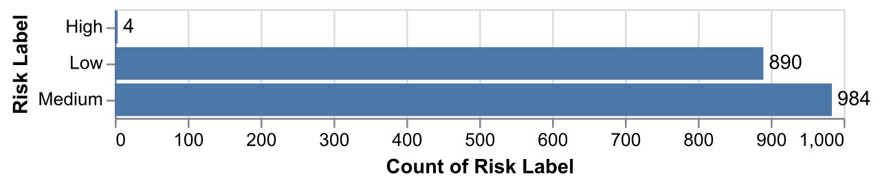
Fig. 1 Histogram of the Risk Label highlighting severe class imbalance
The second issue was that there might be some features hidden from the raw data. Feature engineering techniques are necessary to augment the value of existing data and improve the performance of our machine learning models. This will be described in further detail in Section 3.5.
3.3 Data Augmentation
A major challenge was the imbalanced nature of data, particularly with regard to the class of interest (High Risk). We had only four observations of the High Risk API class in our training set which was insufficient for the models to learn how to predict this class effectively. We attempted these approaches:
Synthetic Data generation
Bootstrapping
Oversampling (SMOTE)
For Synthetic Data generation, while it is able to generate new numerical data, the nature of the technique did not allow us to generate columns for text data, such as response data and response metadata. For Bootstrapping, while it was easy to implement, and the overall data size did increase, the underlying distribution and imbalance in Risk labels was not handled.
Hence, we used the imblearn package for Oversampling. It is a technique that generates new data by ‘clustering’ the data points based on the risk labels and generating new samples based on their ‘neighbours’ information. This technique gave a balanced dataset with sufficient representation of High risk class for further modeling (Fig. 2).
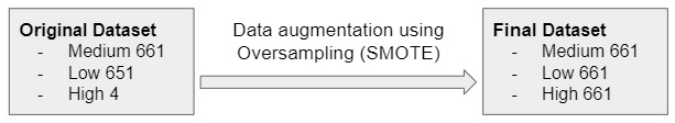
Fig. 2 Transformation of imbalanced training data set to a balanced one
3.4 Evaluation Metric and Acceptance Criteria
As per our discussion with TeejLab, we understood that it is critical to correctly identify the High Risk classes, while also ensuring that not too many Low and Medium risk labels are incorrectly classified as High Risk.
Thus, we selected Recall 1 as the primary evaluation metric to optimize the models and to maximize the correct identification of High Risk labels. We also considered f1-score as the secondary evaluation metric to ensure that not too many data points were incorrectly classified.
It was agreed that Acceptance Criteria would be: Recall \(\geq\) 0.9.
3.5 Feature Engineering
As mentioned above, the dataset consists of 18 variables, which include identity numbers, strings and text. Based on our domain understanding, it is essential to extract and/or engineer several features - (1) PII and FII extraction, (2) quantify exposure frequency, (3) quantify risk associated with server location, and (4) imputation of security test.
PII and FII are crucial pieces of personal and financial information that can be used to identify, contact or even locate an individual or enterprises 3. It is imperative that they are transmitted and stored securely. The team attempted several techniques to extract this information, including Amazon’s Comprehend, PyPi’s piianalyzer package, and Microsoft’s PresidioAnalyzer. However, PresidioAnalyzer was ultimately chosen as it had high accuracy, was transferable between both PII and FII and was cost-free. By using PresidioAnalyzer on the “sample_response” column and defining the pieces of information to pick up on for PII and FII (See Appendix A), we created two binary columns of whether PII and/or FII is exposed by the API endpoint (Fig. 3).
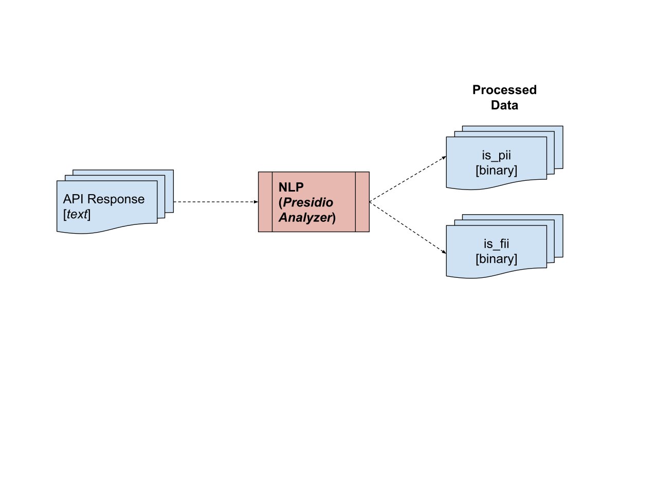
Fig. 3 Extraction of PII and FII from API Response to create two new columns
Second, we had to quantify the exposure of sensitive information. This sensitive information was present in two columns - “parameter” and “response_metadata”. These columns have a format similar to a python dictionary (key-value pairs). The former refers to request data while the latter refers to HTTP response headers.
To quantify exposure, we counted the number of keys exposed per API endpoint (See Fig. 4 below). In addition, there were specific security response keys that, if exposed, could lead to a security breach. As such, we extracted 12 security response keys, and created binary columns of whether each of these 12 keys were present or absent (bottom right of Fig. 4). See Appendix A for the list and description of the 12 keys.
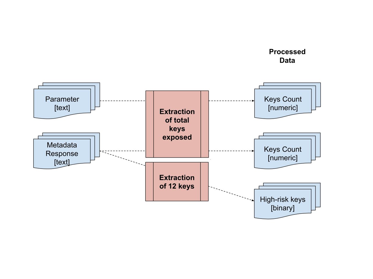
Fig. 4 Extraction of exposure frequency in parameter and metadata response column
Third, we had to quantify the risk associated with the server location (country). Apart from ensuring high loading speed of the API endpoint if it is situated near the user, the infrastructure, technology and the governance associated with the country could also impact the API’s security. As a proxy, our team has used the Network Readiness Index 4. It is an annual index that quantifies the impact of digital technology.
Finally, API exposes application logic and sensitive data, and has unique vulnerabilities and security risks. Ideally, each endpoint would contain all five security tests (as seen in Fig. 5) which TeejLab deems as crucial. However, it is unreasonable for third parties such as TeejLab to request for a temporary shutdown of these API. Based on our discussion with TeejLab, we determined that should a test not be present, it would be deemed as low risk as there was no concern warranting a request for a security test. To capture the subtle difference between a test that passed and a test that was missing, we assigned a value of 0.5 to denote that the specific test was missing, 0 to denote that specific test was employed and passed, and 1 to denote that specific test was employed and failed (Fig. 5).
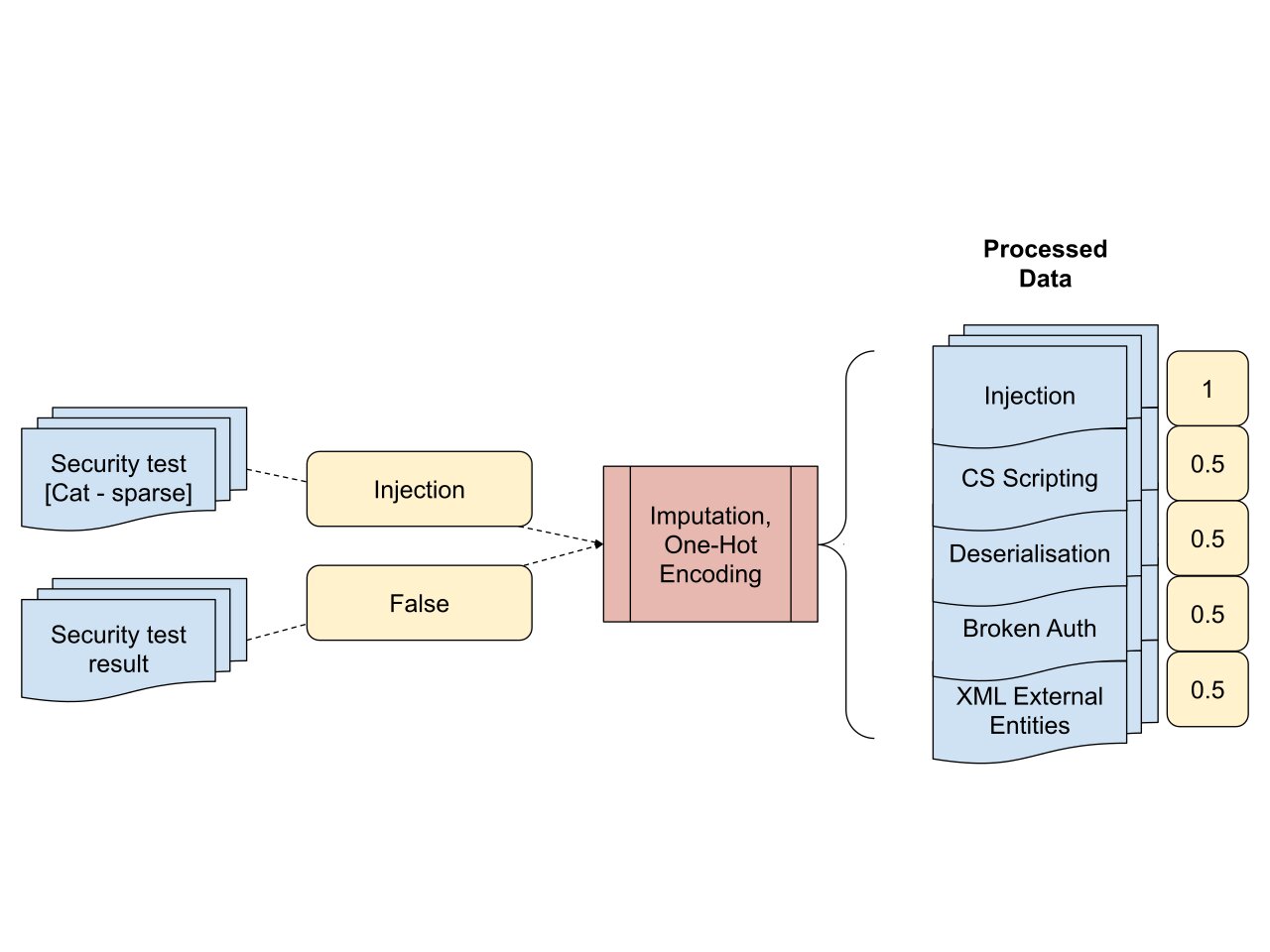
Fig. 5 An example of the processed data when the input is “Injection test failed”
3.6 Supervised Learning
As the risk labels (target column) were provided by TeejLab, we approached this problem as a Supervised Machine Learning task. We attempted the following algorithms:
Logistic Regression
Tree-based Models: Decision Tree, Random Forest, XGBoost, CatBoost
K-Nearest Neighbors (KNN) and Support Vector Machines (SVM)
For each of these models, they were initially trained using the processed data set without any feature engineering. However, the maximum recall value was 0.75. Hyperparameter optimization did not lead to any significant improvement in performance of models. At this stage, Logistic Regression was selected for integration into the prediction pipeline. This is due to its high interpretability and its performance was on par with more complex models. (Refer to the unbolded section of Fig. 6 for comparison). Please refer to the technical report for more details.
To improve the scores, we reviewed the information being captured by the input features, transformed all existing columns and created new features as described in Section 3.5. This resulted in an improvement in the model performance by more than 20% (a high recall score of 0.99), which exceeded the partner’s expectations.
Due to feature engineering, the feature set increased from 17 to 53. Thus, we employed feature selection to reduce the dimensionality yet ensuring that our recall score remains high. We attempted the following algorithms:
Recursive Feature Elimination (RFE)
RFE with Cross Validation (RFECV)
SelectFromModel()
RFE is a backward selection method which recursively considers a smaller feature set, RFECV works similarly but eliminates features based on validation scores, while SelectFromModel selects the relevant features based on feature importance. We ultimately chose RFE as it was the most consistent and resulted in the greatest dimensionality reduction from 53 to eight. The improvement of recall score is provided in Fig. 6.
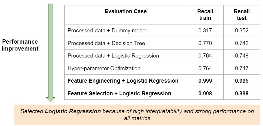
Fig. 6 Improvement of training and testing recall scores via Featuring Engineering and Feature Selection.
- 1
It is the number of true positives divided by the number of true positives plus the number of false negatives”. In our case, it is the ratio of the number of cases correctly identified as High Risk compared to the sum of the cases correctly identified as High Risk and the number of cases incorrectly identified as High Risk when it is actually Low or Medium Risk.